



reporting
Copying and pasting campaign data into a spreadsheet is the worst hour of an analyst’s week. It’s boring, it’s easy to get wrong, and a single misaligned paste can quietly poison a whole month of reporting.
This is a 7-step method for building an automated marketing dashboard in Google Sheets. Setting it up the first time takes a while because you’re learning the pieces. Once you’ve done it once, rebuilding it for a new client takes under 30 minutes.
Every report starts with clean, centralized data. You want all the raw information inside one Google Sheet, split into a separate tab per source. Decide which sources feed the report, then pull them in.
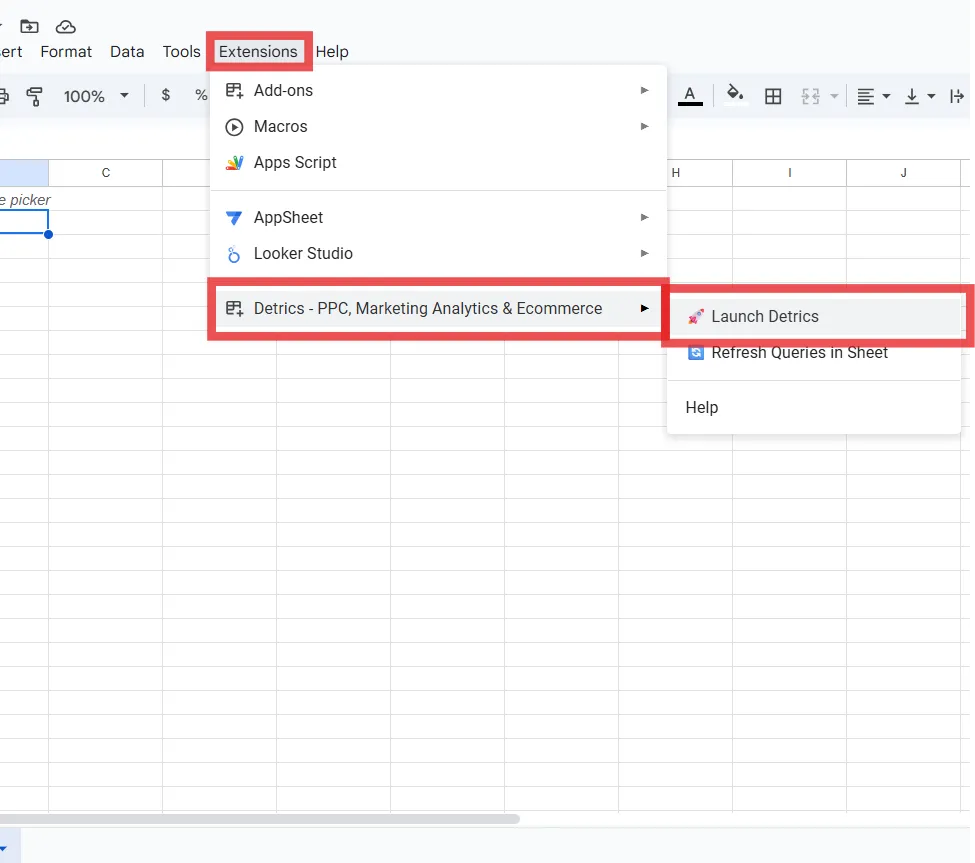
Connectors like Detrics pull data from Meta Ads, Google Ads, Shopify and the rest straight into your Google Sheet. If you already have Detrics installed, open a new Spreadsheet and launch the sidebar from Extensions > Detrics > Launch to start setting up automated data flows.
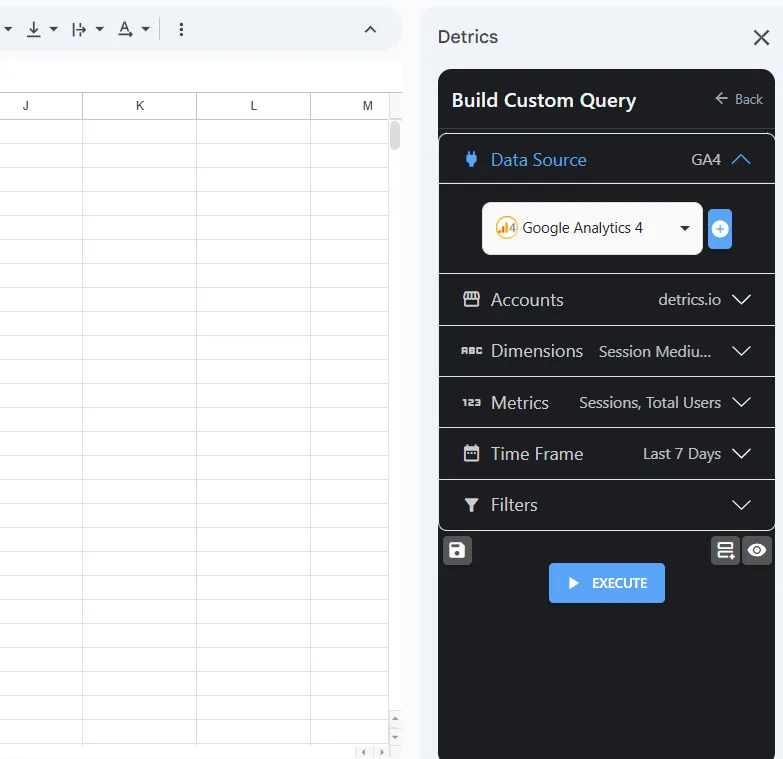
Set up a tab for each source: “Raw_Meta”, “Raw_Google”, “Raw_Shopify”. Schedule the updates daily and manual downloads stop being your problem.
Tip: color-code your columns so you can tell raw connector data apart from anything a formula produced. In the example below we use ARRAYFORMULA to stamp the channel name into each tab. ARRAYFORMULA applies a formula to a whole row or column at once, so you never have to drag it down again when the data refreshes and the table gets longer.
The headers in black carry raw information straight from the connector, exactly as the platform sent it. The column in blue, where we define the channel, is generated by a formula.
=ARRAYFORMULA( IF( ISBLANK(A2:A) , , "Meta" ) )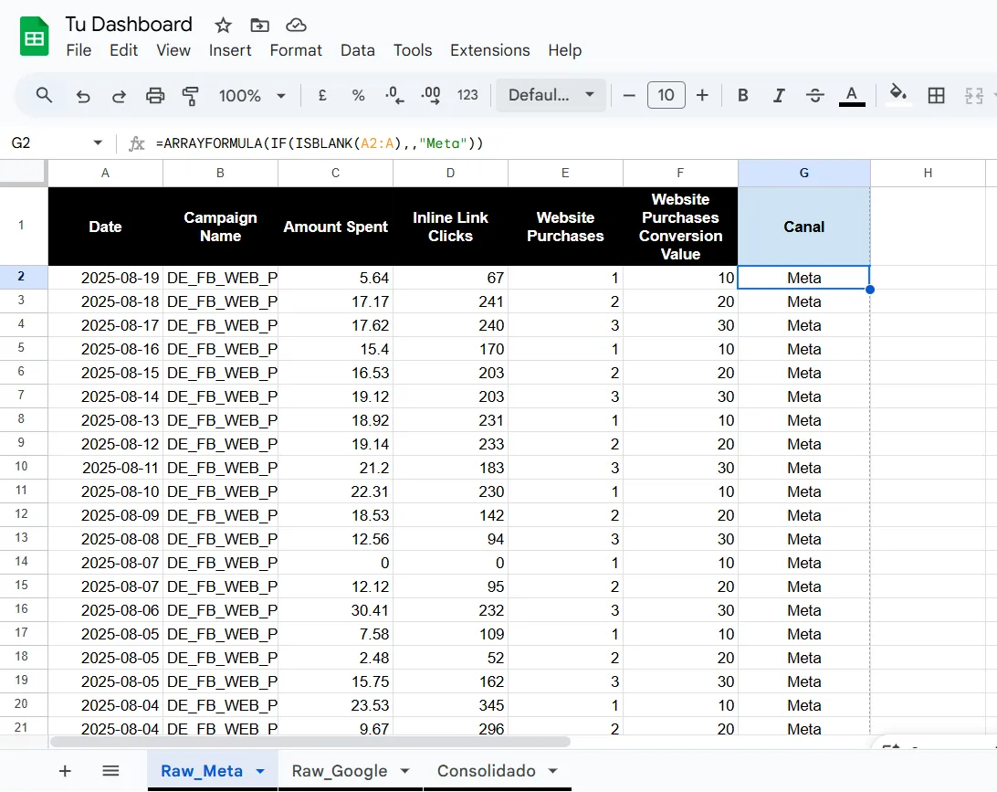
Without a connector, the manual route still works. Export each platform’s report (a CSV of Meta Ads campaign data, say) and paste it into its tab.
Key advice: keep the column structure identical across every tab. A typical order is Date, Campaign, Investment, Clicks, Impressions, Conversions, Revenue. In Detrics you can reorder columns after running your queries with the Sort & Order fields function.
Your data now sits in separate tabs. Next you merge it into one master table. Create a new tab called “Consolidated”.
With everything in a single table, your summary formulas (sums, averages) point at one range instead of five. That one decision removes most of the fiddly work later on.
If all your raw data tabs have exactly the same columns in the same order, VSTACK is your best option. This formula “stacks” data ranges on top of each other.
In cell A1 of your “Consolidated” tab, write:
={'Raw_Meta'!A1:G1; VSTACK('Raw_Meta'!A2:G; 'Raw_Google'!A2:G)}{'Raw_Meta'!A1:G1; ...}: This takes the headers from one of your tabs.VSTACK(...): Vertically stacks all the data (without headers) from the Raw_Meta and Raw_Google tabs.QUERY is SQL inside Google Sheets. You can select, filter and sort with it, which makes it the most flexible tool in this whole build.
Important: the columns in Raw_Meta and Raw_Google have to be in the same order. If they aren’t, the consolidated table will silently misalign, which is the kind of bug you find three weeks later in a client meeting.
To unify, you can use a construction with curly braces . In cell A1 of “Consolidated”, write:
={QUERY('Raw_Meta'!A:G, "SELECT * WHERE A IS NOT NULL");
QUERY('Raw_Google'!A2:G, "SELECT * WHERE A IS NOT NULL")}
{... ; ...}: The curly braces and semicolon stack the results of the two QUERY queries."SELECT * WHERE A IS NOT NULL": Selects all columns (*) but only from rows where column A (the date) is not empty. This avoids bringing blank rows.Most people skip this step. It is the one that decides whether you can still maintain the sheet in six months.
A named range is a label you attach to a set of cells. Instead of writing the investment column as Consolidated!D2:D1000, you call it “Consolidated_Investment”.
SUM(Consolidated_Investment) tells you what it’s summing. SUM(‘Consolidated’!D2:D1000) does not. When the table grows past row 2000, every formula pointing at the named range follows it without you touching anything, and because the reference is descriptive rather than positional, dragging formulas around stops producing off-by-one disasters.
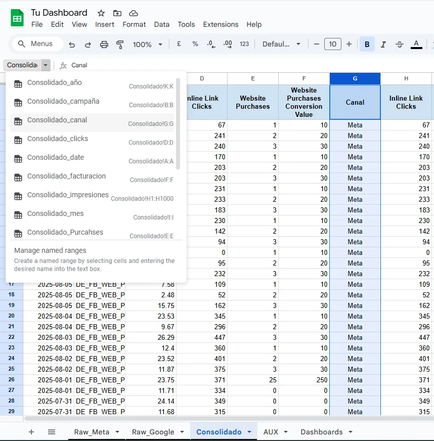
With the table built and the ranges named, you can start on the part people actually look at.
Create a new tab called “Dashboard”. This is the only tab you show stakeholders, so keep it narrow and focused on the results you or your client care about.
Lay out a simple table listing your most important metrics, and leave the result cells empty for now. Order them by business importance rather than by what’s easy to calculate:
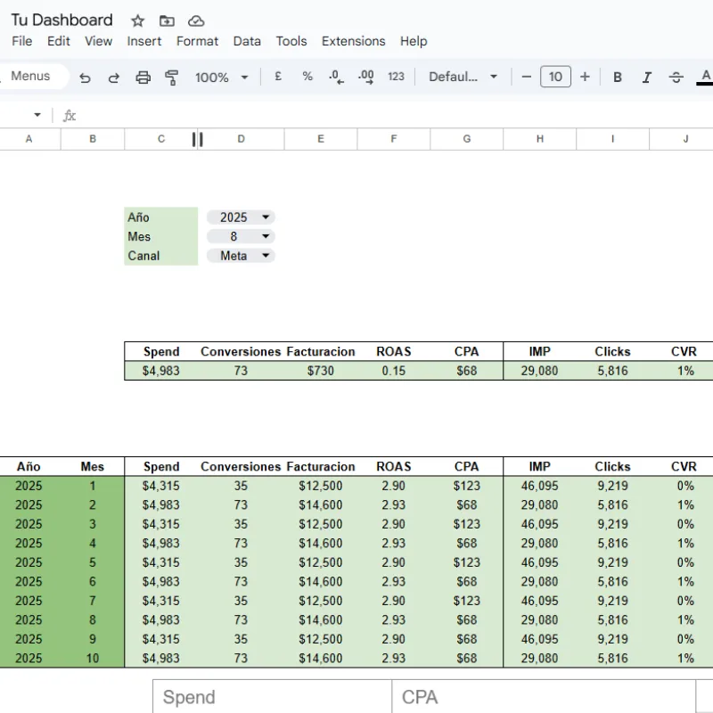
A static report answers one question. Add a dropdown to filter by country, client or channel and the same sheet answers a dozen.
=UNIQUE(Consolidated_Channel); =UNIQUE(Consolidated_Country)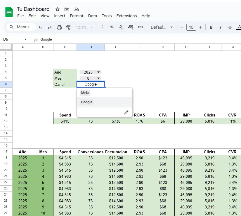
Now you wire the logic to the display, using summary formulas that read from the named ranges and the dropdown filter.
The workhorse here is SUMIFS (SUMAR.SI.CONJUNTO in Spanish), which sums a column only where conditions in other columns are met.
Example: In the cell where you want to display the total investment of your campaigns, write:
=SUMIFS(Consolidated_Investment, Consolidated_Channel, C1)Change the Channel in the dropdown and the investment figure updates on its own. Repeat the same logic for Clicks, Conversions and the rest.
We also lean on the SUM and FILTER combination:
=SUM(FILTER(Consolidated_Investment,Consolidated_Channel=C1))With this combination, SUM will only sum the data that FILTER filters, and in this case, it’s when the channel from the consolidated base equals cell C1 (the dropdown we created)
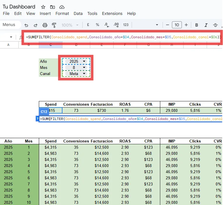
The metrics worth reporting are usually ratios: CPA, ROAS, CTR. Ratios involve division, and division throws #DIV/0! the moment the denominator hits zero, which happens on any day with no conversions or no clicks. Besides looking sloppy, those errors break the charts that reference them.
Wrap the formula in IFERROR.
Example for CPA (Cost per Acquisition):
=Investment_Cell / Conversions_Cell=IFERROR(Investment_Cell / Conversions_Cell, 0)IFERROR reads as: “try this calculation, show the result if it works, and if it errors show this other value instead” (a 0, in our case). Your dashboard stays clean on the bad days as well as the good ones.
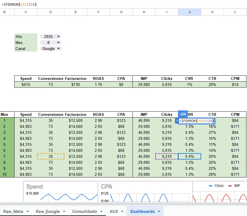
The report has to work. It also has to be pleasant to look at, or people won’t linger on it.
Use your company’s colors, or the client’s. Set up conditional formatting (Format > Conditional formatting) so cells turn green or red depending on whether a value moved the right way, which is especially useful on things like CPA variation.
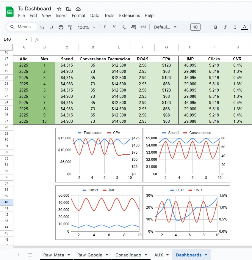
You’ve gone from a folder of disconnected exports to one sheet that refreshes itself: raw tabs per source, a consolidated table stacked with VSTACK or QUERY, named ranges holding the references together, and IFERROR keeping the ratios from blowing up on a zero-conversion day.
The point of all this is not that it saves you a few hours a week, although it does. It’s that the numbers stop being something you assemble and start being something you interrogate. Which is the part of the job worth doing.



Free plan forever
Bring your marketing data into Google Sheets, Looker Studio, BigQuery or Claude. No credit card required.

